Cell Cultivation

Hint

The sample project and datasets used in this quick-guide can be downloaded here .

Download and Start the Toolbox

Download the latest version of the Toolbox for free from the Portal Downloads section, extract the folder from the .zip file, enter it and open IdentificationTool.exe by double-clicking.

Note

This is an exportable desktop version, which does not require installation. You agreed upon the terms and conditions upon registration. However, you can always get back to them using either the homepage or the documentation button inside the toolbox.

On the start screen you see several objects – use the Unlock Console in the center to login by entering your User Name and the chosen Password.

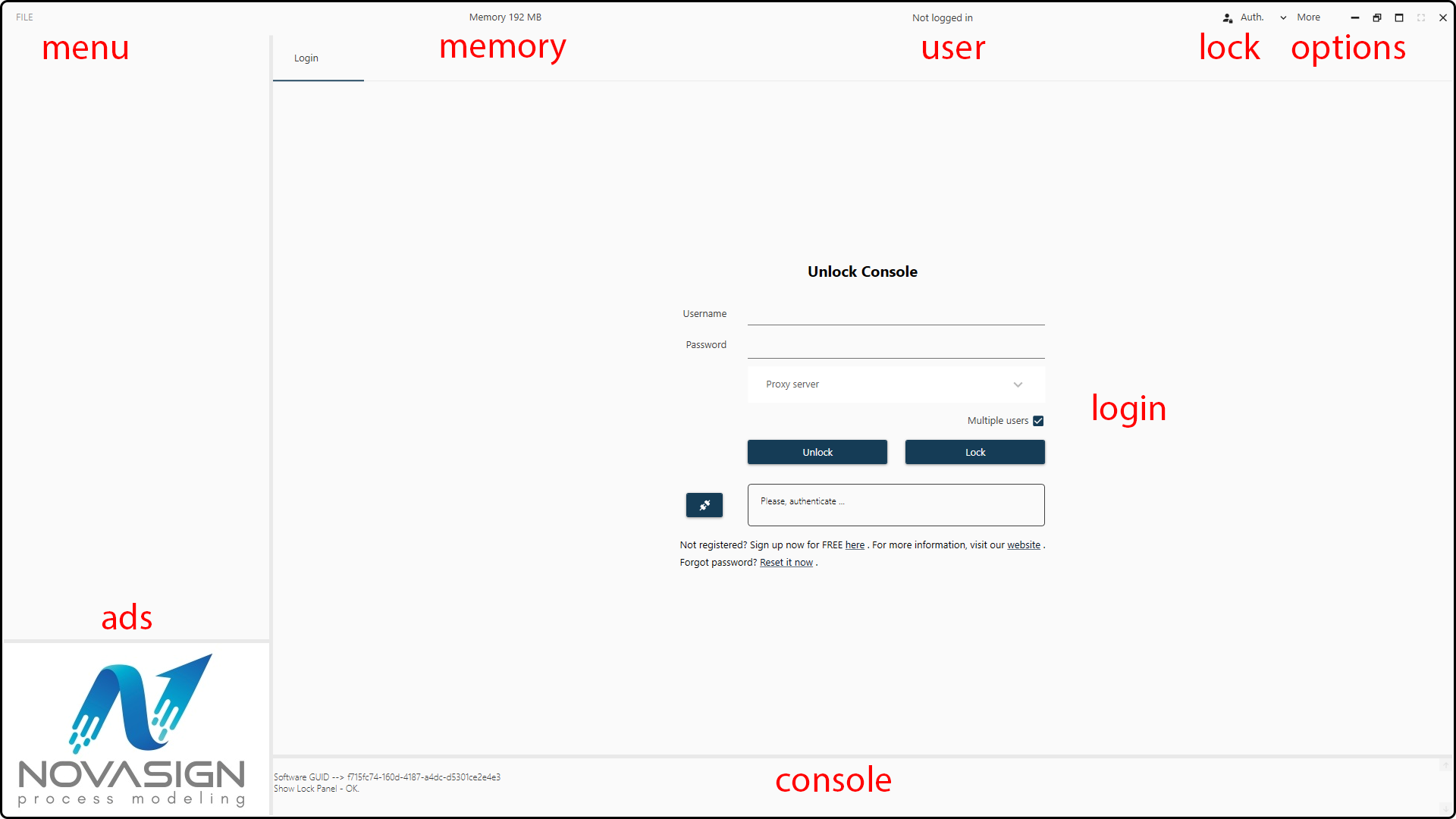
Figure 33. Start screen of the Hybrid Modeling Toolbox.

If you don’t have a user name, you have to sign up by clicking at the hyperlink – you will be forwarded to our registration form. Once you registered and unlocked the console, you can start using the Toolbox and exploring your data.

Note

You can lock the console at any time by clicking on the Auth. button in the main bar. By doing so, no changes can be done in the Toolbox until you unlock the console again.

Dataset structure

Warning

To ensure the proper functionality of the hybrid modeling toolbox, the data you want to import has to be structured properly.

Note

You can use the provided data set as the reference template and to better understand the required data structure.

What follows are requirements and recommendations for the datasets to be imported:

• Valid data formats are .xls, .xlsx, .csv, .txt., .dat and .mat.

• Arrange your data such that each variable is represented by one column and that each observation (usually a time point) corresponds to one row.

• Do not use letters in rows, apart from the first row; this will cause import and calculation problems.

• Likewise, attach new runs/experiments after the last row of the last run.

• Put the Time variable (its name is not of importance) in the first column for each data set.

  Note

  This is not mandatory, but recommended. By default, when setting up your models, the Time column is selected as the first one (but this behaviour can be changed).

  Note

  Use an adequate time resolution for your online variables. If you model is a microbial process do not use less than 3 minutes. Your model calculation will just take much longer without any benefits. For mammalian processes a time grid of 15 to 30 minutes is recommended.

• Assign the Run ID to the last column. Again, this is not mandatory, but recommended.

  Error

  The Run ID must be a number/numerical value. Other values rather than a number will result in an error.

• Name the variables with a header in the first row of the data, but do no use special characters, e.g., square brackets and spaces. Spaces and square brackets will still allow you to import and plot your data, but will cause problems when used as modeling inputs.

Good variable name	biomass(g/L)
Poor variable name	biomass (g/L) or biomass [g/L]

• Use bioprocess units for your parameters to be modeled. Otherwise, the mass balances are wrong, e.g., sampling and reactor volume (volume in L; masses in grams; concentrations in g/L).

• For interpolation, ensure all data series contain more than a certain number of valid (i.e. not missing) values. For example:

  • For linear interpolation: at least 2 values are required

  • For cubic robust interpolation: at least 3 values are required

  • For interpolation with Hermite polynoms: at least 3 values are required

• If your dataset contains missing values, define an invalid number for all empty fields in the data, e.g., the software standard is often ‘-9.999’.

Warning

Empty cells are also supported in case you want to leave it blank. But its value will be replaced by NaN (Not A Number).

• Make sure to have a valid value (other than -9.999 or blank) for each first line of each variable in each run you want to model! Otherwise, the system will not work!

• Split the data in a training/validation (used for setting up/fitting the model) and a test set (used for checking the model performance).

Note

You should import at least two files; one for training/validation and one for testing. It is also possible to upload a separate file for each run and assemble the training/validation and test runs together afterwards.

Example

A typical data structure before import:

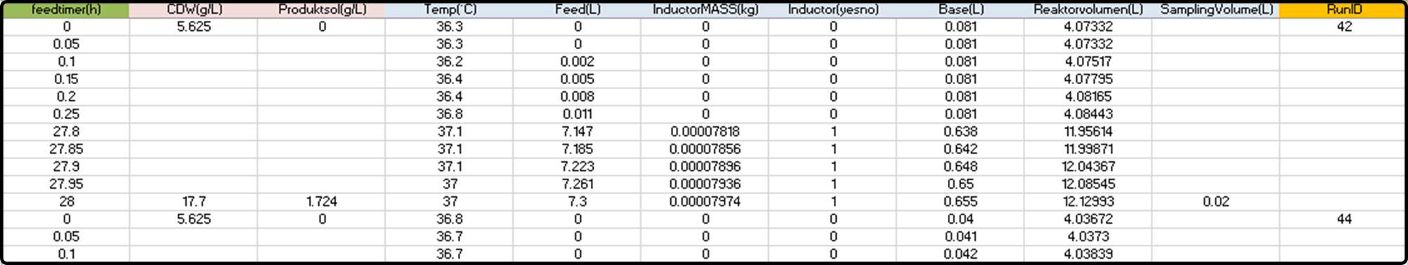
Note that some variables are available at a high frequency (online variables), while some others are only sparsely available (offline variables) and have many missing values/blank cells.

Correctly formatted data for modeling:

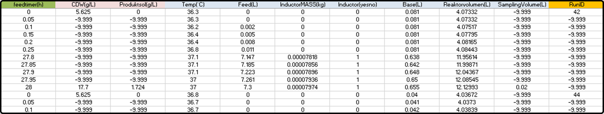
Blank cells have been filled with the invalid numerical value -9.999.

Create a New Project and Import Data

Typically, the first step is to start a new project with FILE – New and entering a project name in the following dialog. We choose the name Test_project four our data.

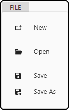
Figure 34. Items of the FILE menu.

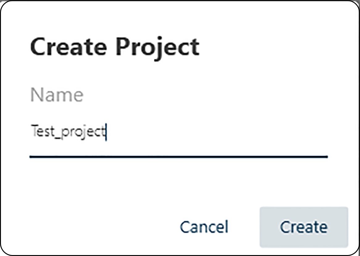
Figure 35. Entering a project name.

Alternatively, choosing Open loads an existing project and Save or Save As saves the current project.

Our project appears in the left column of the project explorer as well as the new menu PROJECT in the main bar. We choose PROJECT – Add Data and the Microsoft Excel file format .xlsx as import format.

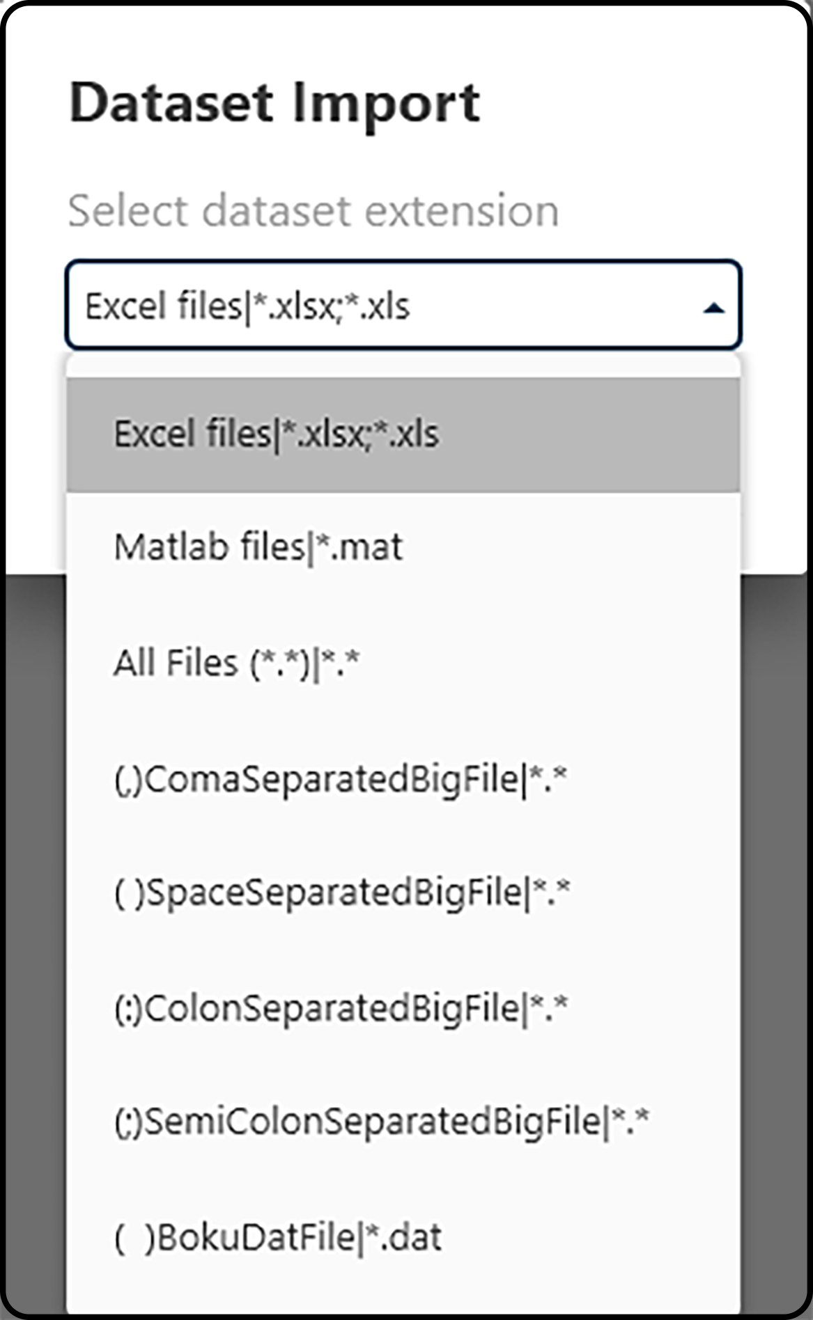
Figure 36. Choosing a file format to be imported.

In the following import window we select the downloaded Train.xslx file.

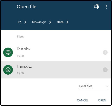
Figure 37. Choosing a file to import.

Note

The three vertical dots in the right upper corner of the open file dialog box can be used to change the drive. Furthermore, only files of the previously chosen file format are shown in the open file dialog.

Once selected, a new window will open, where the properties of the data sheet have to be specified.

• Name: a name for the data; we choose TrainingData

• Decimal separator: the character used as decimal separator, typically either a dot . or a comma ,; in the present case the latter one.

• Sheets: which sheet(s) to import; we keep the default, as the file contains only a single sheet.

• Header row: the row containing the header; here it’s the first row.

• Columns: the columns of the dataset to import; we keep the default (all columns)

• Range: range (in the row-sense) of the data; we keep the default 2 to 2788 (all rows).

• Series names: The column containing the Run ID; here it’s the last column F11. Make sure that the Run ID variable contains a numerical value in the first row of each run, followed by blanks or invalid numbers (e.g. -9.999) for all other rows of this run.

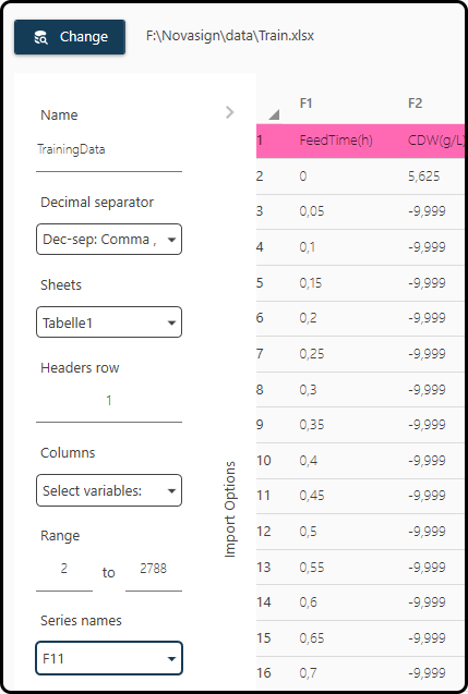
Figure 38. Import dialog. A correct setting of several parameters is of high importance.

Note

Repeat these steps for all data files you want to import – in the present case also for the file Test.xlsx, which contains the test dataset (which we give the name TestData). Take care that you choose the same properties for all data sets.

Finally, both the training and the test dataset will appear in the left column of the project explorer in the Data section.

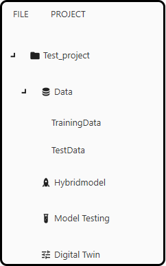
Figure 39. Data section after successful import.

Inspecting and Plotting the Data

Click on the respective data set in the Data section on the left shows the Table View and Plotting Panel tab (to be switched in the main bar). Possible import errors are displayed in the lower-left panel.

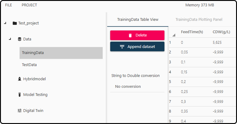
Figure 40. Data table view.

Different options how to deal with the respective data set(s) are available, e.g. datasets can be combined (appended) with the Append dataset button or deleted using Delete.

Error

Deleting datasets being used in other models or plots might result in errors, so this option should be used with care.

In the plotting panel the data can be visually inspected.

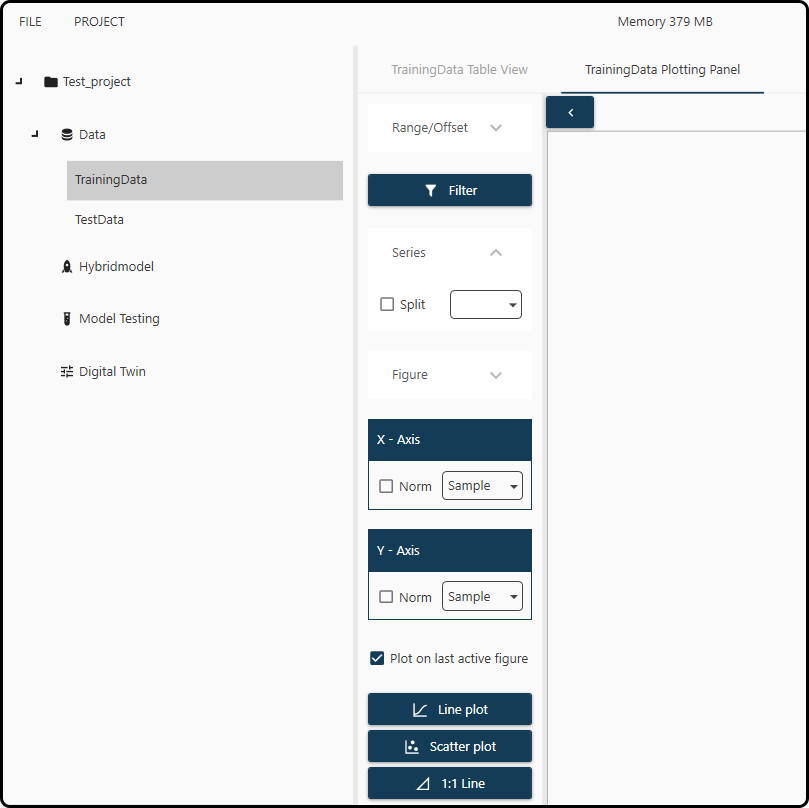
Figure 41. Plotting panel for data visualization.

A few selections are necessary to plot. For demonstration purposes we decide to plot the Cell Dry Weight (in g/L; variable name CDW(g/L)) versus time (variable FeedTime(h)) for all runs in the RunID column.

• Range/Offset: restrict the visualization to certain rows (observations) of the data.

• Filter: specify invalid values and prevent them from being plotted. For the present data set checking both boxes and entering the invalid number -9.999 is necessary:

  

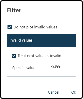
  Figure 42. Specifying and filtering invalid values.

  Note

  This function is activated when the box is green.

• In the Series field, the variable used to split/separate the runs/experiments must be specified. Every time the numerical value in this variable decreases, a new run is assumed by the Toolbox. For our data, we check the box and select the FeedTime(h) variable.

• In the Figure section we can choose a title, legend and axes annotations (but we keep the default).

• In the X-axis and Y-axis section we choose our variable pair to be plotted. We choose FeedTime(h) for the horizontal (\(x\)) and CDW(g/L) for the vertical (\(y\)) axis.

• Finally, we can decide on the type of plot (either a line or a scatter plot with or without a 1:1 line – we choose the first option). Checking the Plots on last active figure option plots multiple figures (e.g. a scatter- and a line-plot) on the same sheet (not used here).

We finally get as a result

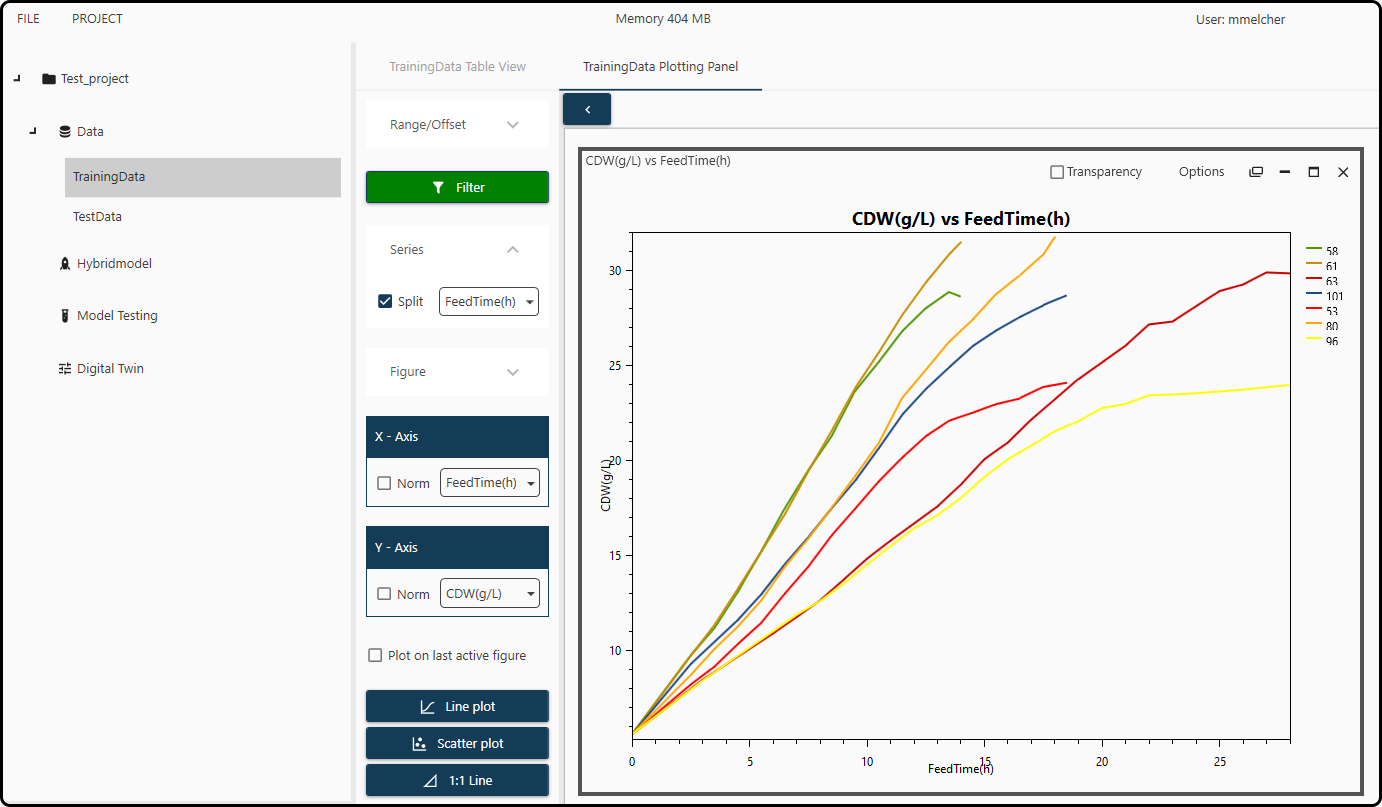
Figure 43. Plot of the cell dry weight CDW(g/L) versus FeedTime(h) for each of the 7 runs in the training set.

Additional plotting options (such as positioning the legend, exporting in various file formats or axes formatting) are available after undocking the figure and clicking on the Options menu of the figure.

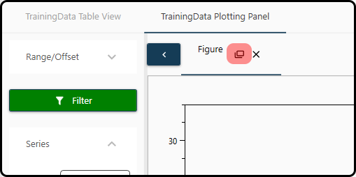
Figure 44. Undocking a figure.

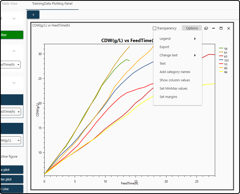
Figure 45. Further plotting options are available in the Options menu.

Building a Hybrid Model

Generally, there are two types of modeling, often called black box or white box modeling. Black box models are purely data-driven approaches, for which no further process knowledge is needed. This kind of modeling is relatively easy to apply and has good interpolation abilities. However, once the model is applied to data not within the design space, it lacks the ability to extrapolate and the model performs poorly. On the other hand, white-box models are based on first principles and therefore are a suitable match for extrapolation. Since they solely assume a mechanistic trend and do not account for empiric phenomena, also their predictability often ends up inaccurately.

One way to exploit the advantages of both modeling approaches is called hybrid modeling. Hereby it is possible to benefit from the positive aspects of both previous modeling approaches, black box and white box, and make up for their respective drawbacks. The hybrid modeling approach often yields a more robust model compared to one that only uses one of these techniques. In contrast to simple black or white box models, hybrid models are able to describe the whole process and not only the endpoints. As a result, the dynamics and deviations of a process can be incorporated. A graphical example of how a hybrid model structure may look like and how the different parts are integrated is given below.

Typically the online measurements serve as inputs to the data-driven (black box) model – here an artificial neural network (ANN) is used – and its outcome(s) will be fed as rates into the mechanistic (white box) part of the hybrid model. The outcomes of the latter are in the present case the target variables biomass and and product concentration. Furthermore, a correction for the sample volume (if necessary) can be taken into account.

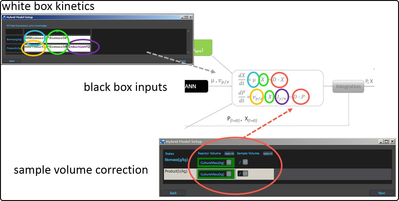
Figure 46. Serial structure of a hybrid model.

The goal is to develop a hybrid model that performs well on new data and predicts its target variable(s) accurately. To achieve this, an appropriate model complexity must be chosen to avoid a phenomenon called overfitting – a higher number of hidden layers, hidden neurons or a higher number of iterations will only improve the model performance (on new data) to a certain point. Hereby, the training error will continue to decrease, while the model’s performance on new data will get worse. In practice, the available data are often (randomly) split into a training/validation set and a test set (external validation). The model is built on the training and applied on the validation part (internal validation) to determine an optimal modely complexity. Once this is found, the final model is applied on the test set to estimate its performance on new, unseen data. An scheme of how the model complexity affects the model performance, with respect to the training, validation and test set, is given below.

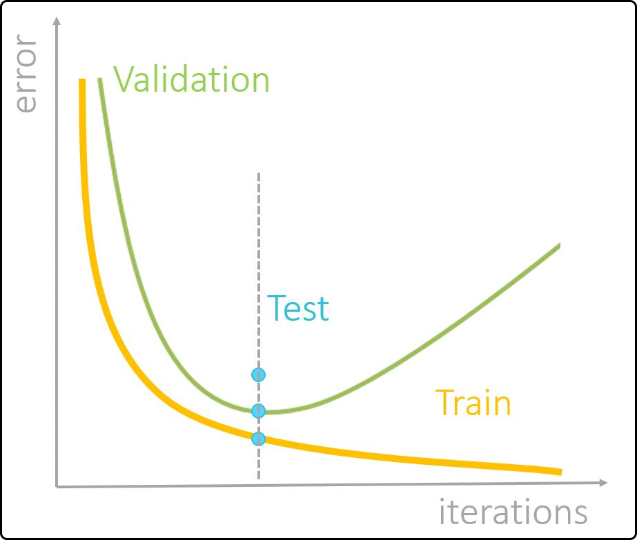
Figure 47. Profiles of training, validation and test error with increasing model complexity.

To create a hybrid model with for our data sets, we use PROJECT – Add Hybridmodel. We get a dialog, in which we have to enter a model name in step 1 – we choose HybridModel

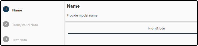
Figure 48. Choosing a name for the hybrid model.

In step 2 we select the data set(s) to use for training and validation by drag and drop from the left to the right subwindow. We choose our TrainingData. Note that it is possible to add more than one data set.

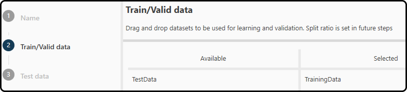
Figure 49. Selecting the data for training and validation.

In step 3 we do the same for the test data (in the Toolbox: TestData). Again it is possible to add more than one data set.

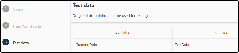
Figure 50. Selecting the data for testing the model performance.

In step 4 the user is asked to specify the outputs (responses, targets), which are the quantites to be modeled/predicted. In our example we choose the cell dry weight in g/L – CDW(g/L) and the soluble protein Productsol(g/L), which we drag and drop from the left (where all variables in our dataset are listed) to the right part of the window.

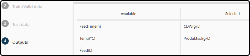
Figure 51. Selecting the variables to be modeled.

In the optional step 5 variables can be specified for correcting the volume of the process, e.g., in the case of fed-batch or sampling a column for the volume compensation can be given. It is important to provide these variables in kg or L to ensure the correct calculation. For the reactor volume provide the cumulative volume over time; for the sample volume the volume of the extracted sample at each time point must be used (do not provide a cumulative volume here). We use the variables Feed(L), ReactorVolume(L) and SamplingVolume(L) for both output variables.

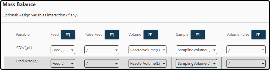
Figure 52. Optionally variables can be specified to correctly consider the mass balance.

In the next window (step 6), the variables to be used for building the data-driven black box part (the ANN) of the hybrid model – selection is done again via drag and drop from the left to the right side. We use Temp, Feed(L), InductorMass(mg) and Inductor(yesno). Do not select those variables, which were specified as outputs in step 4.

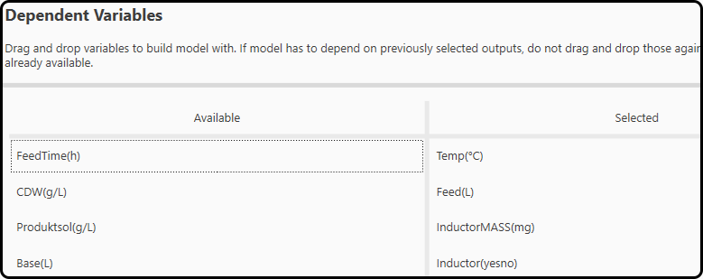
Figure 53. Drag and drop the inputs to the neural network in this step.

In step 7 we have to setup some technical details of the black box (ANN) model and set some further options. Note that the chosen parameters might not be the optimal ones – modeling is typically an iterative process, in which the effect of these parameters on the results obtained for this specific data set at hand have to be found out by trial and error. What follows is a short description of (most of) the available options and some recommendations on the parameter settings.

• Model and Neural Network Settings

  • ANN hidden layers: this defines the number of hidden layers of the neural network. In most cases a single layer is sufficient.

  • Number of nodes: this defines how many nodes your hidden layer(s) should consist of. A good number to start with is the amount of ANN inputs -1 for a low to

    moderate number of inputs, but can be much smaller than the number of inputs for data sets with many predictors.

  • Hidden Layer TF: this will allow you to set the transfer (activation) function of the hidden layer. Most of the time ‘Tanh’ (tangens hyperbolicus) works best.

  • Output Layer TF, this sets the transfer function of your output layer of the neural network. It is recommended to use a linear trasfer function here.

  • ANN input SNS: this allows you to choose the scaling/normalization/standardization method for the ANN inputs, ensuring fair conditions. This is necessary in order to take the different orders of magnitude of the ANN inputs into account. Zscore scaling (subtraction of the mean and division by the standard deviation) is a good choice often used for machine learning tasks.

• Optimizer Stopping Criteria

  • Max. Iterations: this defines the maximum number of performed iterations before a new Jacobian is set. May strongly vary from dataset to dataset.

• Data Preprocessing

  • Volume variables: here the type of interpolation used for the volume variable, to correct for the increasing volume in a fed-batch and the volume reduction

    due to sampling is specified.

  • Model-based variables: this sets the interpolation type of the input parameters for the model and the ANN.

  • Sens. Train. modeled variables: this sets the interpolation type of the target/state variables.

    Note

    Remember that a minimal number of observations for each interpolation type is required (typically 2 or 3 per run/experiment).

  • Dataset ‘Time’ index: this defines the column number containing the Time variable. Note that the column number minus 1 has to be specified here. If the

    Time variable is located in the first column, 0 has to be entered here, if the Time variable is in position 5, 4 must be entered etc.

  • Integrative dt: defines the time step/temporal resolution of the model. It is recommended not to use a value below the minimum online sampling time here.

  • False data value: as in the plotting panel earlier, this defines the false/invalid data value assigned to empty cells/missing values.

• Train Options

  • Num. best models: this parameter determined how many of the best performing models per start point will be kept/available to report,

    after the model-building process.

  • Num. Starts: this number defines how often the ANN is initiated with new random weights, to find the global minimum. The more starts, the more likely

    it is that a global minimum of the loss function is found.

  • Num. Steps: defines how often the Jacobian Matrix is reset (5 is a good number to start with).

  • Num. of Boots: defines how often to shuffle the data with the set Train/Val ratio. If for example 10 runs are available and a 0.8 ratio is set,

    45 different combinations are possible (using a number of 5 to 10 boots typically gives a good guess of the model performance).

  • Train/Val ratio: splits your training/validation dataset into a training and validation part according to this ratio. If e.g. the training/validation set

    consists of 10 runs and a 0.8 ratio is chosen, 8 runs go to the training and 2 to the validation set.

  • Recommended setup: for 4-10 runs: 0.75, for 10-30 runs: 0.8, for > 30 runs: 0.9.

For the present example we use a 1 hidden layer neural network with 6 hidden units, tanh as hidden layer TF, a linear output layer TF, Z-score scaling and 100 iterations. We use linear interpolation for all variables, specify a 0 in the Time variable field (as the FeedTime is located in the first column), a dt (time grid) of 0.1 and specify -9.999 as the false data value. We keep the best 3 models, use 5 random starts, 1 step and 7 boots with a training/validation ratio of 0.95 (resulting in splits with just 1 run in the validation part).

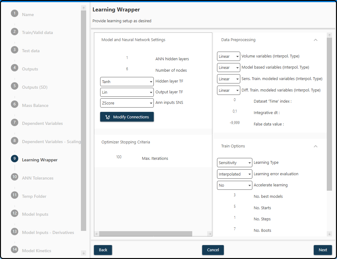
Figure 54. A summary of the model settings for the present data set.

In step 8 the black box part of the hybrid model is defined. All variables previously added to consider in the model-building are available. More input panels can be added if needed and also simple mathematica functions of the variables (e.g. \(log(x)\)) are possible. The variables are color-coded:

• Green variables: these are the state variables to be modeled, but can also be use in the ANN as inputs. They will only be used in the first iteration for a good approximation of the starting point.

• Purple variables: these are modeling parameters (at best critical process parameters, which can be controlled by the operator) and will be used for each iteration.

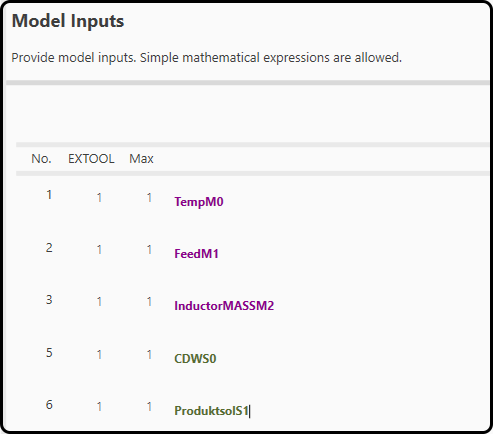
Figure 55. Variables used as inputs to the neural network.

After setting up the black box part, the kinetics for the white box part of the hybrid model are needed in step 9. Generally, this mechanistic part is obtained by either process knowledge or the literature.

Note

For help ask us via the Novasign Portal.

In the present project, the white box part uses the state variables (CDWS0), the outcome from the black box (variables prefixed with an ANN, namely ANNCDWS2 and ANNProductsolS3) and our process knowledge in respect to the product formation (InductorM3, contains either 0 for no product formation or 1 for product formation), based on the following equations

Note

\[\begin{split}\begin{matrix} \frac{dX}{dt}= {\color{Red} \mu \cdot X} - D\cdot X\\ \frac{dP}{dt}={\color{Red} \upsilon _{p/x}\cdot X\cdot I_{y/n}}-D\cdot P \end{matrix}\end{split}\]

Note that the terms including the dilution \(D\) are automatically included (if specified in step 4).

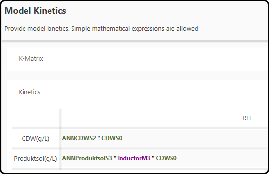
Figure 56. Kinetic expressions used in the hybrid model.

Once all the settings are done, the hybrid model appears under the chosen name (HybridModel) in the corresponding section in the left column of the project explorer. Clicking on it reveals all options previously selected in various tabs (Learning Wrapper, Model Inputs, Kinetics, Datasets and Others).

Figure 57. The hybrid model screen with all our previously defined settings.

The learning (or fitting) process is started by choosing Start near the top of the screen. During learning the Toolbox switches to another view showing the current boot, start and iteration number as well as the obtained model errors and plots of the predicted versus measured values for all output variables.

Depending on the size of the data (both rows and columns), the model complexity and the available computational power, learning might take from seconds to several hours. For our small demonstration example 1-2 minutes can be expected. Lerning can be interrupted at any time using the Stop button. Note that learning can be accelerated by setting accelerate learning to ether ParFor or Tasks in the first tab of modeling options. Learning is then performed on multiple cores (if available on the machine).

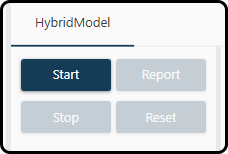
Figure 58. Start the learning process by pressing the Start button.

Once the learning process is finished, a model report can/should be generated using the Report button (which is only available after learning). This allows to select one or more models as final models and the assess the model quality. Depending on these results, one might wish to export models e.g. to the Digital Twin or to start over using different settings.

Pressing Reset before a report is generated disposes the modeling results, but allows to change all the input parameters (e.g. the neural network architecture to explore more complex models or the, the model inputs or kinetics to view alternative model etc.).

Figure 59. Switching between the model options (upper icon) and (if available) the modeling results (lower icon).

Evaluating the Results

After the learning process has finished, a report for the models is created via clicking the Report button. In the Report Model Selection window one or more models can be selected for further inspection. For each boot (tab) and random start (subwindow) up to 2 times the previously defined number of models (3) is listed in the half of the window – the top 3 models with lowest training and the top 3 with lowest validation error (\(MSE\)). Either all or none of these models or a subset of them according to certain criteria can be selected (also a completely manual selection of models is possible by checking the box(es) to the left of the model(s).

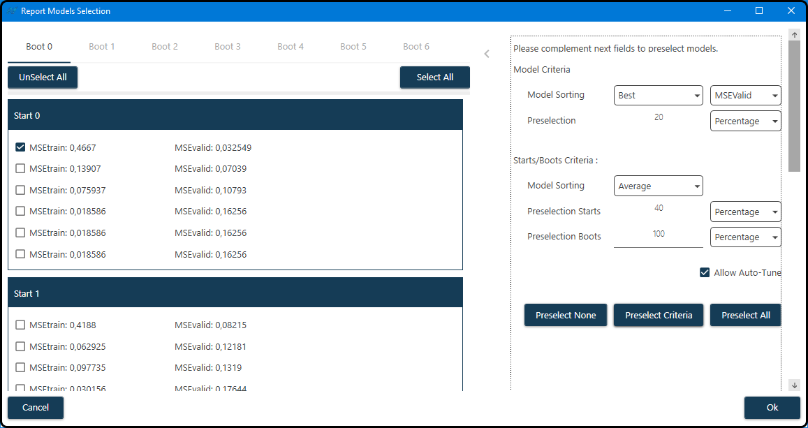
Figure 60. Selection of models according to certain quality criteria.

As shown in the figure, we first sort the models according to their \(\text{MSE}_\text{validation}\) (validation mean squared error) and keep the top 20% of these models for each boot and start. Using only these remaining models, each boot/start combination is characterized by the average \(\text{MSE}_\text{validation}\) of these models and the models of the 40% best starts (and all of the boots) are kept.

Note

After entering suitable values for the selection criteria, the button Preselect Criteria must be clicked in order to apply these criteria.

Now the report is available by switching from the Hybrid Model to the Report tab.

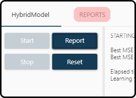
Figure 61. Clicking on the Report tab will allow to inspect the selected models graphically.

In the reports section all previously created reports are accessible via the drop-down menu. Clicking on the Quality Report icon below shows the quality metrics for all selected models, whereas in the Plots 2D section models can be visualized in many ways.

Figure 62. The Quality report and Plot 2D icons.

Plotting can be controlled via 5 tabs: * Plot Types: select the type of plot(s), the error measure to plot and control the model sorting * Train/Validation: plotting of the training/validation runs yes/no (checkbox) * Test: plotting of the test runs yes/no (checkbox) * State Variables: which state variables to plot * Models: select the models to visualize (all or only a subset of those models selected before)

In most cases we leave the defaults, but in plot types we select the \(\text{RMSE}\) as an error measure and choose Plots Global as sorting strategy; in the models section we select all models and choose Plot at the bottom.

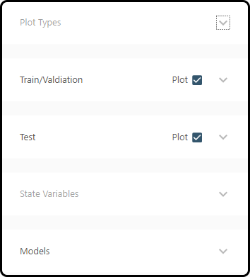
Figure 63. 5 menu items for plot selection and options.

The result for each model is finally presented in a separate tab – models are sorted according to their error with better models being shown first. For both outputs – \(\text{CDW(gl)}\) and \(\text{Productsol(gl)}\), each in a row – scatterplots of the predicted versus measured values and the model predictions versus time in form of line plots are shown for the training and validation data and for the test set. Overall and per-experiment quality measures (here: \(\text{RMSE}\)) are given below each plot, whereas the plots and the underlying data can exported with the Export button above each plot. Further options to change the appearance of the plots (e.g. colors) are also available.

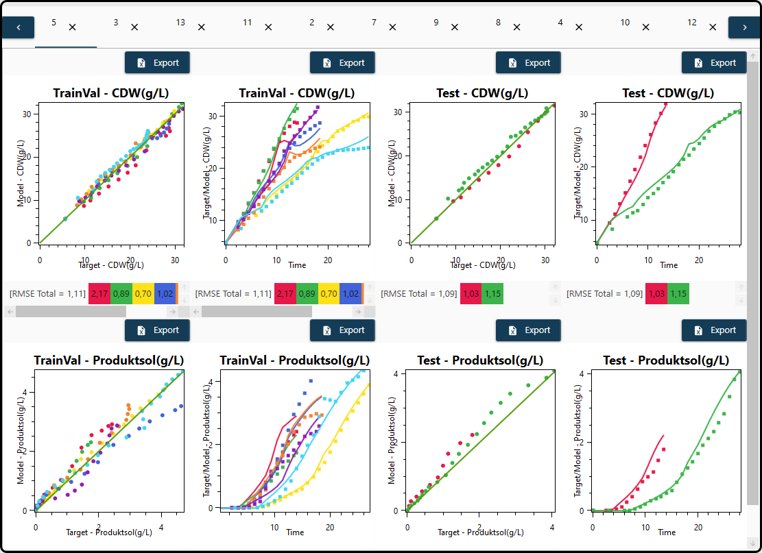
Figure 64. Model performance visualization – each model in its own tab, each outcome has its own row.

One would probably go through all the plots of the 14 models listed in the Models section by switching between the different plotting tabs and

• return to the model setup if the model quality is not sufficient. A different architecture of the neural network model, further inputs, changing hyperparameters such as the number of iterations or a different mathematical formulation of the mechanistic part of the hybrid model might improve the model performance significantly.

• select some final models and calculate and visualize an averaged model, in which the model predictions are averages of the single models’ predictions. For that purpose the models to be averaged have to be selected in the Models section and Plot avg. (plot averaged model results) must be chosen at the bottom. For averaged models also prediction intervals are available and plotted by default (deselection is possible in the State variables section). In the present example we might choose models 3 and 5 to form a single averaged model.

  

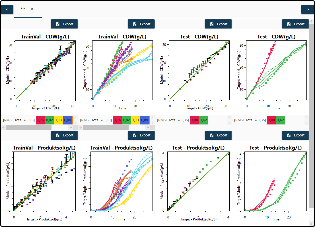
  Figure 65. Visualization of an averaged model consisting of two single models including prediction intervals as error bars.

  Note that the name of the tab of an averaged model contains the model numbers of the single models.

• export a model (a single one or an averaged model) to the digital twin to further explore the design space for optima etc. Therfore, use the Export button near the right upper corner of the screen, select the destination (one of Digital Twin, Inputs Cluster, Sensitivity Analysis and Model Test) and models to export and press Export in the following dialog.

  

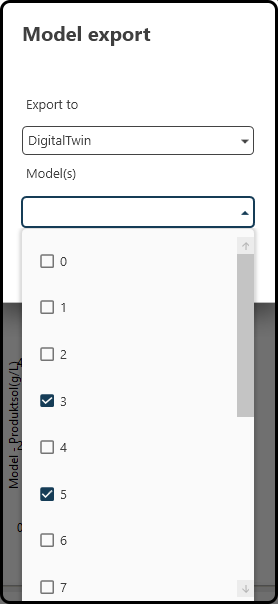
  Figure 66. Exporting a (single or averaged) model to e.g. the digital twin.